Wednesday, December 17, 2014

Excel VBA: Get source data GetSourceData

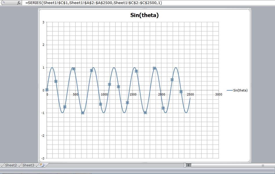
After searching a lot for the solution of this problem, I want to introduce it. For charts, MS Excel does not has a native function to get the source range address for series collection, but we can -with a trick-  get some useful information about the source range using string processing.

The following two pictures show the layout of series collection formula. I noticed that sometimes I get the first layout and sometimes I get the other one (I don't know exactly when I get each one). The difference between them is just the quotation marks of sheet name. The series collection formula has four data:

(1) Data series name: represented by address or string 
(2) Independent variable (x-axis) values: represented by address or defined name
(3) Dependent variable values (y-axis) represented by address or defined name
(4) Index of data series (read only value)

The first layout (with quotation marks):
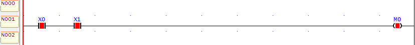
The second layout (without quotation marks):
The following code demonstrates how to get source sheet name for the second layout (Excel 2007)

Sub GetSeriesCollectionData()

' Get the formula of the first data series
SeriesCollectionFormula = Charts("Chart1").SeriesCollection(1).Formula

' Some string processing...
StartPos = InStr(SeriesCollectionFormula, "(")     'Index of first "(" found in the string
EndPos = InStr(SeriesCollectionFormula, "!")    'Index of first "!" found in the string

' Extracting the name of source worksheet using Mid function
SourceWorkSheet = Mid(SeriesCollectionFormula, StartPos + 1, EndPos - StartPos - 1)

'Display the source work sheet in a message
MsgBox ("The name of source work sheet of this chart is : " + SourceWorkSheet)

End Sub


Saturday, October 11, 2014

PLC logic operations


The following are some simple logic operations for PLC programming. X: Input, M: Output. Simulations are conducted on Fatek PLC simulator.

If X0=1 and X1=1 then M0=1

Table of probabilities:


X0
X1
M0
0
0
0
1
0
0
0
1
0
1
1
1


If only X0=1 and X1=0 then M1=1

Table of probabilities:

X0
X1
M1
0
0
0
1
0
1
0
1
0
1
1
0


If X0=1 or X1=1 then M3=1

Table of probabilities:

X0
X1
M3
0
0
0
1
0
1
0
1
1
1
1
1


 If  one only of contacts X0 or X1 equals 0 then M5=1

Table of probabilities:

X0
X1
M5
0
0
1
1
0
1
0
1
1
1
1
0


Saturday, July 12, 2014

Tools sorting method for 5S

In workshops and production lines we always need to sort our hand and power tools and keep them in fixed places to reach them quickly and easily without wasting time and effort in looking for them and this what is called 5S: Sort, Straighten, Shine, Standardize, and Sustain. The following are some concepts showing how to allocate a fixed place for each tool.

First of all, imagine that we have two pieces of tools or objects like in the image below.


The first method is to use a foam insert or a vacuum-formed plastic inserts. This method is the best as it provides good fixing and cushioning for tools.


The second method is to make a monochromatic color shadow for objects with high contrast (white board and black shadow). This shadow board is easy to recognize from far distances.


The third method is to make a thick outer contour lines for objects. 


The forth method is to print colored pictures for objects, so the objects will be placed on their pictures. Pictures may be 1:1 scale, or may be a reduced or enlarged scale. It is preferred to have a picture with an orthogonal view for the object as it will be viewed on the board.


The fifth method is to use name labels only, so tools will be placed above or under their labels. This method is the worst method to use for sorting tools specially if a tool has more than one name, or if there are different tools having the same name but different sizes (like wrenches, screw drivers, drill bits,... etc).  


The sixth method is stick labels on both tools and board. Each label will have a unique code.

Method number 7 is to use samples or demos. This method is almost used with consumable objects like tubes, hoses, tapes, screws, paints, electric terminals, wires, cables, plugs, blades, drill bits, ...etc. For example, in case of adhesive tapes, you can cut a small square piece of each tape and paste it on the board. 


Notice that more than one of these methods can be used at the same time. 


Thursday, June 19, 2014

"CoolProp" fluid thermodynamic properties Excel add-in

After searching over the internet for "Engineering Equation Solver EES package for Excel", I came through some other alternatives for Engineering Equations Solver thermodynamic properties calculator:

RefProp: Open source (free)

CoolProp: Open source (free)


XProps: Commercial package


1. CoolProp


Download the package (zipped file) from the following link


http://sourceforge.net/projects/coolprop/files/CoolProp/


1.1. Installation in Excel:


Unpack the zip file you downloaded to any folder on your hard disk "New folder"

Open "New folder\dist_temp\windows_superpack\Excel and DLL" and copy its contents

Create a folder in your partition C: "C:\CoolProp". It should be placed in C: partition even if it is not your system (default) partition.

Paste the copied files to the folder "CoolProp" you have created

Copy CoolProp.xlam to the default directory of Excel add-ins. To know the default directory of Excel add-ins in your PC, just create a new book and save it as Excel add-in file (*.xlam). Copy the address and discard saving this file.


Open Excel options and select add-Ins


Press "Go..." button shown highlighted by the red box in the image above and you will get a window like below. Check the "CoolProp" add-In so it will be automatically loaded each time you open excel.


It is done...


This is a demo after installation of add-in (see equation in equation bar). You can use cell references instead of direct values for sure.


and this is a snapshot after I have implemented this add-in in my Ref Analysis add-in


1.2. Comparison with EES:


1.2.1 Fluid properties


For real fluids the following are the available properties in EES and CoolProp (units displayed are as displayed in EES):


Property name
EES
CoolProp
Accentric factor
Conductivity [W/m.K]
Cp [kJ/kg.K]
Cv [kJ/kg.K]
Density [kg/m3]
Dipole [debye]

Ek_Lj [K]

Enthalpy [kJ/kg.K]
Entropy [kJ/kg.K]
Fugacity [kPa]

IntEnergy [kJ/kg]
isIdealGas [-]

MolarMass [kg/kmol]
P_crit [kPa]
P_sat [kPa]
Phase$

Prandtl [-]

Pressure [kPa]
Quality [-]
Sigma_LJ [m]

SoundSpeed [m/s]
SpecHeat [kJ/kg.K]
SurfaceTension [N/m]
T_crit [C]
T_triple [C]
Temperature [C]
V_crit [m3/kg]
Viscosity [kg/m.s]
VolExpCoef [1/K]

Volume [m3/kg]


1.2.2 Reference state

The reference state used in CoolProp is International Institute of Refrigeration IIR reference which assumes that the specific enthalpy of saturated liquid fluid Q=0 at 0 C equals 200 kJ/kg and the specific entropy at the same conditions equals 1 kJ/kg.K . From the other side EES uses three reference states IIR, Normal Boiling Point NBP, and ASHRAE, but they can be manually-correlated by adding constants in CoolProp.

1.2.3 Properties abbreviations (names) in CoolProp

Property name
Properties CoolProp codes
w
Thermal conductivity
L
Cp
C
Cv
O
Density
D
Specific enthalpy
H
Specific entropy
S
Internal energy
U
Molar mass
molemass
Critical pressure
pcrit
Pressure
P
Quality
Q
Sound speed
A
Gibbs function
G
Surface tension
I
Critical temperature
Tcrit
Triple temperature
Ttriple
Triple pressure
ptriple
Minimum temperature
Tmin
Ozone depletion potential
ODP
Temperature
T
Dynamic Viscosity
V

Later, I will update this post and illustrate the notations, units.